Query optimization is the art and science of making ClickHouse queries run faster, use less memory, and consume fewer CPU cycles. In ClickHouse, a well-optimized query can be 100-1000x faster than a poorly written one. Optimization involves understanding the query execution pipeline, leveraging indexes effectively, and writing queries that align with ClickHouse's architecture.
📊
Query Analysis
Use EXPLAIN to understand how ClickHouse executes your queries and identify bottlenecks.
🗂️
Index Strategy
Leverage primary keys, skipping indexes, and bloom filters to drastically reduce data scanned.
⚙️
Execution Pipeline
Understand how ClickHouse processes queries: parsing, optimization, compilation, execution.
💾
Resource Management
Optimize memory usage, CPU utilization, and I/O operations for maximum performance.
The primary key determines sort order and enables range queries. Use low-cardinality columns first to maximize effectiveness.
Reduces data to scan
Enables binary search
Improves cache locality
Index Utilization
ClickHouse has multiple index types: primary key, skipping indexes, bloom filters.
Skipping indexes skip blocks
Bloom filters check membership
Reduce I/O significantly
Memory Optimization
Control memory usage with settings and query tuning.
max_memory_usage limits RAM
Aggregation state compression
Streaming aggregation
JOIN Optimization
Joins are expensive; minimize or eliminate them.
Denormalize data when possible
Use dictionary tables
Filter before joining
🚀 Quick Start: Basic Query Optimization
1. Understand Your Query Performance
-- Get query execution time
SELECT /* ... query ... */ FORMAT JSON SETTINGS max_execution_time = 30;

-- Use EXPLAIN to see query plan
EXPLAIN SELECT * FROM events WHERE country = 'US' AND event_date >= '2026-01-01';

-- Use EXPLAIN PIPE to understand pipeline
EXPLAIN PIPE SELECT * FROM events WHERE country = 'US';

-- Check query statistics
SELECT
    query_id,
    query_duration_ms,
    read_rows,
    read_bytes,
    result_rows,
    memory_usage
FROM system.query_log
WHERE query_kind = 'Select'
ORDER BY query_duration_ms DESC
LIMIT 10;
2. Add an Index to Speed Up Queries
-- Create table without optimization
CREATE TABLE events (
    event_date Date,
    event_time DateTime,
    country String,
    event_type String
) ENGINE = MergeTree()
ORDER BY (event_date, event_time);

-- Query 1: Without index (slow)
SELECT COUNT(*) FROM events WHERE event_type = 'purchase' AND country = 'US';

-- Now add a skipping index
ALTER TABLE events ADD INDEX idx_event_type event_type TYPE set(2) GRANULARITY 4;
ALTER TABLE events ADD INDEX idx_country country TYPE set(2) GRANULARITY 4;

-- OPTIMIZE to rebuild index
OPTIMIZE TABLE events FINAL;

-- Query 2: With index (10-100x faster!)
SELECT COUNT(*) FROM events WHERE event_type = 'purchase' AND country = 'US';
3. Materialized Views for Pre-Aggregation
-- Slow query (recalculates every time)
SELECT
    toDate(event_time) as date,
    country,
    COUNT(*) as count
FROM events
WHERE event_date >= today() - 30
GROUP BY date, country;

-- Fast solution: Pre-aggregate with materialized view
CREATE MATERIALIZED VIEW events_daily_mv
ENGINE = SummingMergeTree()
ORDER BY (date, country)
AS SELECT
    toDate(event_time) as date,
    country,
    COUNT(*) as count
FROM events
GROUP BY date, country;

-- Now query is instant!
SELECT date, country, count
FROM events_daily_mv
WHERE date >= today() - 30
ORDER BY date DESC;
💻 Commands & Tools Reference
EXPLAIN - Understanding Query Plans
-- Basic EXPLAIN
EXPLAIN SELECT COUNT(*) FROM events WHERE country = 'US';

-- EXPLAIN SYNTAX (just parse, don't execute)
EXPLAIN SYNTAX SELECT COUNT(*) FROM events;

-- EXPLAIN PLAN (more details)
EXPLAIN SELECT COUNT(*) FROM events WHERE country = 'US';

-- EXPLAIN PIPE (show data processing stages)
EXPLAIN PIPE SELECT COUNT(*) FROM events WHERE country = 'US' GROUP BY country;
Index Management
-- Add a skipping index
ALTER TABLE events ADD INDEX idx_country country TYPE set(2) GRANULARITY 4;

-- Add a bloom filter index (for IN queries)
ALTER TABLE events ADD INDEX idx_event_type event_type TYPE bloom_filter GRANULARITY 4;

-- Add a minmax index (for range queries)
ALTER TABLE events ADD INDEX idx_timestamp event_time TYPE minmax GRANULARITY 4;

-- Add a tokenbf_v1 index (for string matching)
ALTER TABLE events ADD INDEX idx_message message TYPE tokenbf_v1(256, 2, 0) GRANULARITY 4;

-- Drop an index
ALTER TABLE events DROP INDEX idx_country;

-- List table indexes
SHOW CREATE TABLE events;

-- Rebuild indexes (after ALTER)
OPTIMIZE TABLE events FINAL;
Query Profiling & System Tables
-- View query performance history
SELECT
    query_id,
    query,
    query_duration_ms,
    read_rows,
    read_bytes,
    result_rows,
    memory_usage,
    exception_code
FROM system.query_log
WHERE query_kind = 'Select'
  AND query_start_time >= now() - INTERVAL 1 HOUR
ORDER BY query_duration_ms DESC
LIMIT 20;

-- Find queries that use the most memory
SELECT
    user,
    query_id,
    query,
    memory_usage / 1024 / 1024 as memory_mb,
    query_duration_ms
FROM system.query_log
WHERE type = 'QueryFinish'
ORDER BY memory_usage DESC
LIMIT 10;

-- Monitor active queries
SELECT
    user,
    query_id,
    query,
    elapsed,
    read_rows,
    memory_usage / 1024 / 1024 as memory_mb
FROM system.processes;

-- Table sizes and part count
SELECT
    database,
    table,
    formatReadableSize(sum(bytes)) as size,
    count() as parts,
    max(modification_time) as last_modified
FROM system.parts
WHERE active = 1
GROUP BY database, table
ORDER BY sum(bytes) DESC;
✨ Best Practices
1. Primary Key Design is Critical
❌ Bad
-- High cardinality first (user_id has millions of values)
CREATE TABLE events (
    event_id UUID,
    user_id UUID,  -- HIGH cardinality!
    country String,
    timestamp DateTime
) ENGINE = MergeTree()
ORDER BY (user_id, timestamp);  -- Bad order!
Problem: Poor compression, range queries don't benefit
✅ Good
-- Low cardinality first
CREATE TABLE events (
    event_id UUID,
    user_id UUID,
    country LowCardinality(String),  -- LOW cardinality
    timestamp DateTime
) ENGINE = MergeTree()
ORDER BY (country, toDate(timestamp), user_id);  -- Low-to-high cardinality
-- Requires JOIN every time
SELECT u.name, COUNT(*)
FROM events e
JOIN users u ON e.user_id = u.user_id
WHERE e.event_date = today()
GROUP BY u.name;
Problem: JOINs are slow and memory-intensive
✅ Good: Denormalized Data
-- Denormalize: store user_name in events table
CREATE TABLE events (
    event_date Date,
    user_id UInt64,
    user_name String,  -- Denormalized!
    event_type String
) ENGINE = MergeTree()
ORDER BY (event_date, user_id);

-- No JOIN needed!
SELECT user_name, COUNT(*)
FROM events
WHERE event_date = today()
GROUP BY user_name;
Benefit: 100-1000x faster, no memory overhead
4. Common Anti-Patterns to Avoid
Anti-Pattern 1: Full Table Scans
-- BAD: Reads entire table
SELECT COUNT(*) FROM events WHERE message LIKE '%error%';

-- GOOD: Use appropriate indexes or filter by partition
ALTER TABLE events ADD INDEX idx_message message TYPE tokenbf_v1(256, 2, 0);
SELECT COUNT(*) FROM events WHERE message LIKE '%error%';
Anti-Pattern 2: Functions on WHERE Clause Columns
-- BAD: Function prevents index use
SELECT * FROM events WHERE toDate(timestamp) = '2026-01-22';

-- GOOD: Filter on indexed column
SELECT * FROM events WHERE timestamp >= '2026-01-22' AND timestamp < '2026-01-23';
max_memory_usage_for_user - Total for all user queries
memory_overcommit_ratio - Allow temporary overage for final results
max_bytes_before_external_sort - Use disk for sorting
max_bytes_before_external_group_by - Use disk for GROUP BY
6. Query Rewriting Techniques
Technique 1: Use PREWHERE for Early Filtering
-- PREWHERE filters before reading other columns (saves I/O!)
SELECT user_id, COUNT(*)
FROM events
PREWHERE event_type = 'purchase'
WHERE country = 'US'
GROUP BY user_id;
Benefit: Reduces bytes read by 50-90%
Technique 2: Approximate Queries with SAMPLE
-- Query 10% of data for faster approximate results
SELECT country, COUNT(*) * 10 as estimated_count
FROM events SAMPLE 0.1
WHERE event_date >= today() - 30
GROUP BY country;
Benefit: 10x faster for exploratory queries
🎯 When to Use Query Optimization
✅ Optimize When
Query takes > 100ms
Full table scans happening
Memory usage is high
JOINs are slow
Dashboards are lagging
Reports take too long
Alerts trigger late
Ad-hoc queries are slow
❌ When Optimization Matters Less
One-time batch jobs (correct > fast)
Query already < 50ms
Data is tiny (< 1M rows)
Running on fast SSD with plenty of RAM
Queries run rarely
Not on critical path
🏆 Real-World Results
100x
Faster with Index
Adding proper indexes can speed up queries 100x on large tables
50-90%
I/O Reduction
Using PREWHERE and proper filtering reduces bytes read by 50-90%
10x
Memory Savings
Denormalizing data eliminates JOINs and reduces memory 10x
Dashboard queries taking 5-10 seconds, users frustrated with slow loads
Solutions Applied
Added skipping indexes on country, event_type
Created materialized views for hourly/daily aggregations
Denormalized user data into events table
Used PREWHERE for event filtering
Results
Query Time: 10s → 200ms (50x faster)
Dashboard refresh time: 30s → 2s
User satisfaction: 2/5 → 5/5
Dashboard CPU usage: 80% → 15%
Case Study 2: Real-Time Alerting System
Challenge
Alert queries take 15 seconds, alerts fire late and miss anomalies
Solutions Applied
Added bloom filter indexes on alert_type
Created streaming aggregation views
Optimized memory usage with streaming aggregation
Used sampling for approximate anomaly detection
Results
Alert Latency: 15s → 500ms (30x faster)
Anomalies detected: 70% → 98%
Mean time to alert: 15s → 0.5s
False positives reduced with faster queries
📋 Ready-to-Use Templates
Template 1: Optimized Events Table
-- Well-optimized for analytics
CREATE TABLE events (
    event_date Date,
    event_time DateTime,
    user_id UInt64,

    -- Low cardinality columns first (for primary key)
    country LowCardinality(String),
    event_type LowCardinality(String),
    platform LowCardinality(String),

    -- High cardinality
    session_id String,
    device_id String,

    -- Metrics
    revenue Decimal(10, 2),
    duration_ms UInt32
) ENGINE = MergeTree()
PARTITION BY toYYYYMM(event_date)
ORDER BY (country, toDate(event_time), user_id)
TTL event_date + INTERVAL 2 YEAR;

-- Add indexes for common queries
ALTER TABLE events ADD INDEX idx_event_type event_type TYPE set(5) GRANULARITY 4;
ALTER TABLE events ADD INDEX idx_session session_id TYPE bloom_filter GRANULARITY 4;
ALTER TABLE events ADD INDEX idx_device device_id TYPE bloom_filter GRANULARITY 4;

-- Create materialized view for daily stats
CREATE MATERIALIZED VIEW events_daily
ENGINE = SummingMergeTree()
ORDER BY (date, country, event_type)
AS SELECT
    toDate(event_time) as date,
    country,
    event_type,
    COUNT() as count,
    SUM(revenue) as revenue
FROM events
GROUP BY date, country, event_type;
Template 2: Performance Monitoring Query
-- Monitor query performance
SELECT
    query_id,
    query,
    query_start_time,
    query_duration_ms,
    read_rows,
    formatReadableSize(read_bytes) as read_bytes,
    formatReadableSize(result_bytes) as result_bytes,
    formatReadableSize(memory_usage) as memory_usage,
    user
FROM system.query_log
WHERE query_kind = 'Select'
  AND query_start_time >= now() - INTERVAL 1 HOUR
  AND query_duration_ms > 1000  -- Only slow queries
ORDER BY query_duration_ms DESC
LIMIT 50;

-- Find queries with high memory usage
SELECT
    user,
    query_id,
    substring(query, 1, 100) as query,
    formatReadableSize(max(memory_usage)) as peak_memory,
    max(query_duration_ms) as duration_ms
FROM system.query_log
WHERE type = 'QueryFinish'
  AND query_start_time >= now() - INTERVAL 1 DAY
GROUP BY user, query_id, query
HAVING peak_memory > 1000000000  -- > 1GB
ORDER BY peak_memory DESC
LIMIT 20;
Template 3: Index Analysis
-- Check which indexes exist and their sizes
SELECT
    database,
    table,
    name as column_name,
    type as index_type,
    formatReadableSize(data_compressed_bytes) as index_size
FROM system.data_skipping_indexes
WHERE database != 'system'
ORDER BY database, table, name;

-- Check index effectiveness (via query_log)
-- After adding an index, compare these metrics:
SELECT
    sum(read_rows) as total_rows_read,
    count() as queries,
    formatReadableSize(sum(read_bytes)) as total_bytes_read,
    formatReadableSize(sum(memory_usage)) as total_memory
FROM system.query_log
WHERE query_start_time >= now() - INTERVAL 1 HOUR
  AND query_kind = 'Select';
🔥 Advanced Patterns
1. Query Execution Pipeline Deep Dive
-- Understand each stage with EXPLAIN
EXPLAIN PIPELINE
SELECT country, SUM(revenue) as total
FROM events
WHERE event_date >= today() - 30
  AND event_type = 'purchase'
GROUP BY country
ORDER BY total DESC
LIMIT 10;

-- Execution stages:
-- 1. ReadFromMergeTree - Read data from table with filtering
-- 2. Where - Apply WHERE filters
-- 3. Aggregating - GROUP BY and aggregation
-- 4. LimitStep - LIMIT
-- 5. OutputFormat - Format results
2. Bloom Filter Indexes for Complex Conditions
-- Bloom filter for EXISTS queries
CREATE TABLE events (
    event_id UUID,
    user_id UUID,
    event_type String
) ENGINE = MergeTree()
ORDER BY event_id;

ALTER TABLE events ADD INDEX idx_user_id user_id TYPE bloom_filter GRANULARITY 4;
ALTER TABLE events ADD INDEX idx_event_type event_type TYPE bloom_filter GRANULARITY 4;

-- Now fast: bloom filter eliminates impossible blocks
SELECT COUNT(*)
FROM events
WHERE event_type IN ('purchase', 'signup', 'login');
3. Materialized Views for Complex Aggregations
-- Source table (raw events)
CREATE TABLE events (
    event_time DateTime,
    user_id UInt64,
    event_type LowCardinality(String),
    country LowCardinality(String),
    revenue Decimal(10, 2)
) ENGINE = MergeTree()
ORDER BY (event_type, event_time);

-- Level 1: Hourly aggregation
CREATE MATERIALIZED VIEW events_hourly
ENGINE = SummingMergeTree()
ORDER BY (hour, event_type, country)
AS SELECT
    toStartOfHour(event_time) as hour,
    event_type,
    country,
    COUNT() as count,
    COUNT(DISTINCT user_id) as unique_users,
    SUM(revenue) as revenue
FROM events
GROUP BY hour, event_type, country;

-- Level 2: Daily aggregation (from hourly for efficiency)
CREATE MATERIALIZED VIEW events_daily
ENGINE = SummingMergeTree()
ORDER BY (day, event_type)
AS SELECT
    toStartOfDay(hour) as day,
    event_type,
    sum(count) as count,
    sum(unique_users) as unique_users,
    sum(revenue) as revenue
FROM events_hourly
GROUP BY day, event_type;

-- Now queries are blazingly fast!
SELECT event_type, count, revenue
FROM events_daily
WHERE day >= today() - 30
ORDER BY count DESC;
4. Optimizing JOIN Queries
-- Strategy 1: Use Dictionary table (small reference data)
CREATE TABLE countries (
    country_code String,
    country_name String,
    region String
) ENGINE = MergeTree()
ORDER BY country_code;

-- Create dictionary
CREATE DICTIONARY country_dict (
    country_code String,
    country_name String,
    region String
)
PRIMARY KEY country_code
SOURCE(CLICKHOUSE(TABLE 'countries'))
LAYOUT(FLAT())
LIFETIME(3600);

-- JOIN becomes dictionary lookup (very fast)
SELECT
    dictGet('country_dict', 'country_name', country_code) as country,
    COUNT(*) as events
FROM events
GROUP BY country_code;

-- Strategy 2: Use ALL JOIN (broadcast small table)
SELECT e.user_id, c.country_name
FROM events AS e
ALL LEFT JOIN countries AS c ON e.country_code = c.country_code
WHERE e.event_date = today();
5. Memory-Aware Query Design
-- Monitor and control memory usage
SET max_memory_usage = 1000000000;  -- 1GB limit
SET max_bytes_before_external_sort = 500000000;  -- Use disk if > 500MB
SET max_bytes_before_external_group_by = 500000000;

-- Streaming aggregation for huge GROUP BY
SELECT country, COUNT(*) as count
FROM events
GROUP BY country
SETTINGS
    max_threads = 1,
    max_block_size = 1000000;
📚 Resources & Further Learning
📘 View in Notion
Access this module in your Notion workspace for note-taking and tracking your progress.
After mastering query optimization, you should be able to:
✅ Analyze query execution plans
✅ Design optimal primary and secondary indexes
✅ Create materialized views for pre-aggregation
✅ Optimize JOIN queries or eliminate them
✅ Manage memory and CPU resources effectively
✅ Implement performance monitoring
✅ Achieve 100-1000x query speedups
Ready for Module 7? Next we'll explore Backup & Recovery!
🐳 Hands-on Docker Demo for this Module
A self-contained ClickHouse stack you can run locally. Every step is reproducible; the README below walks through each concept with diagrams and measured outcomes.
cd code-examples/demos/module-6-query-opt
./up.sh        # bring stack up, wait for health
./run.sh       # run the demo (idempotent — re-runnable)
./down.sh      # tear down + drop volumes
📺 Live demo capture
Recorded with vhs: the actual terminal output from ./run.sh running on this very stack.
Animated GIF, ~477 KB. Right-click → open in new tab to view full-size.
✨ Animated concept diagrams
Inline SVG animations — no plugins, native browser playback. Each visualises a key flow this module covers.
Read rows
🗂️ Architecture diagrams
Rendered from the README's Mermaid sources. Click any to open the source SVG full-size.
Q query text p parserSource 20m synthetic events
📚 ClickHouse reference visuals
Curated from the official ClickHouse documentation and engineering blog (and Altinity's docs/blog) — the same diagrams the broader CH community uses to explain these concepts. Click any image to read the source.
ClickHouse Docs
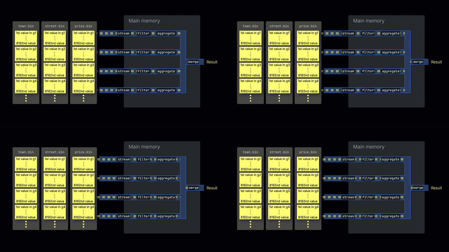
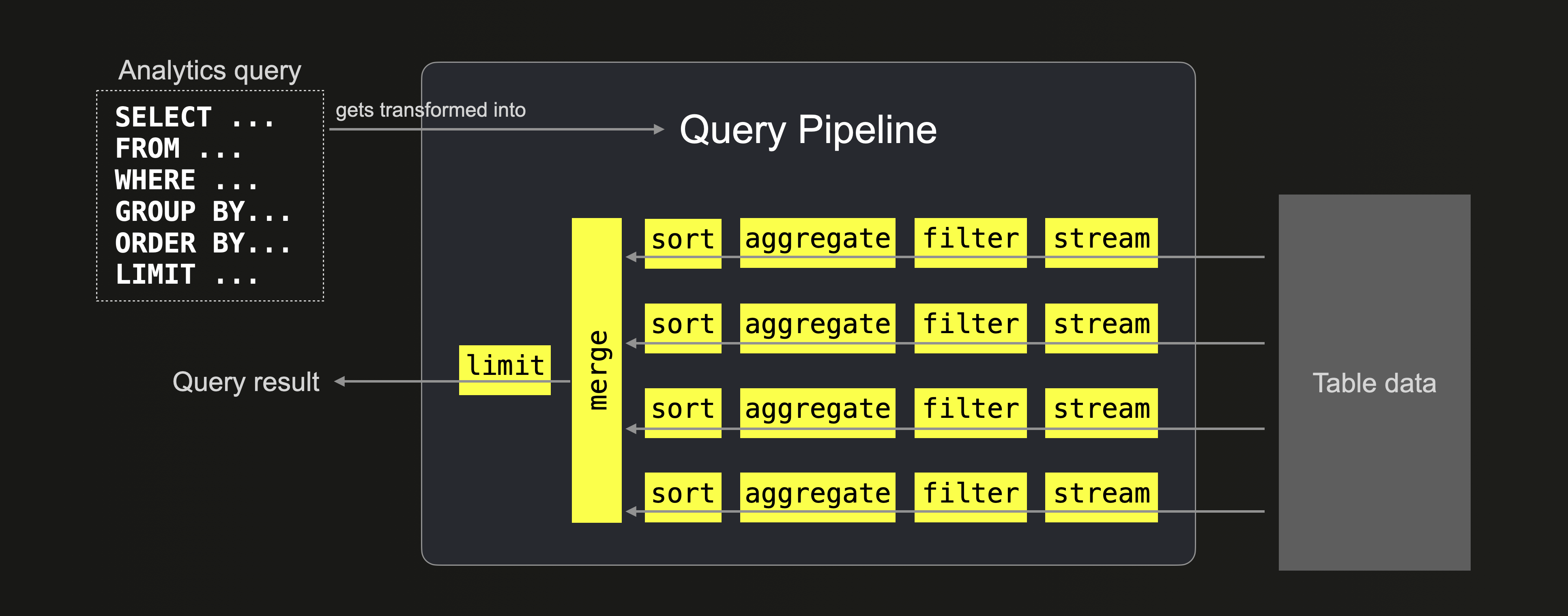
Animated: query splits into parallel processing lanes per CPU core
ClickHouse Docs
Animated: vectorised pipeline pushing chunks through transforms
ClickHouse Docs
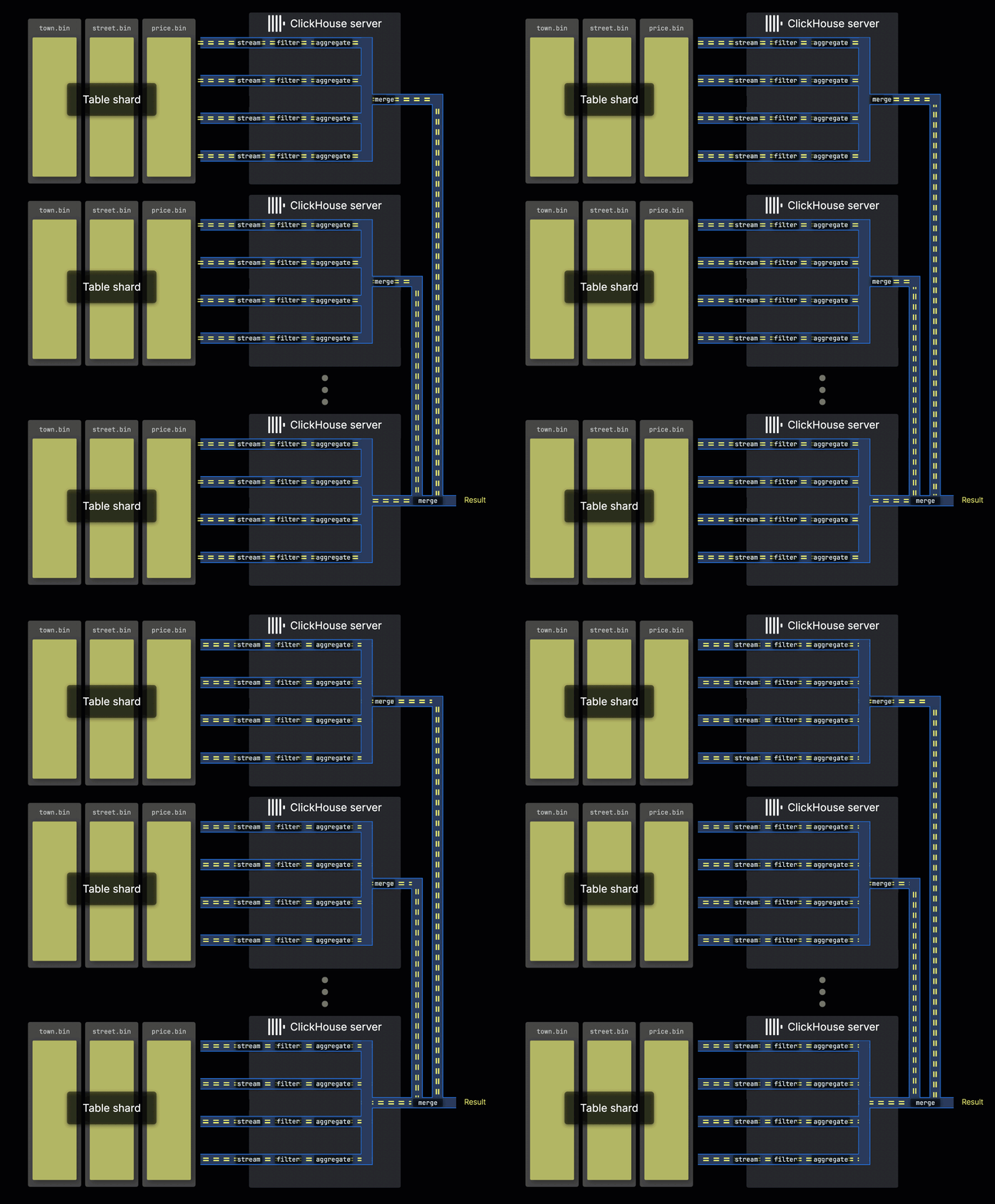
Parallel replicas: query fans out across replicas of a shard
ClickHouse Blog
Processors-and-ports query pipeline (sources, transforms, sinks)
ClickHouse Blog
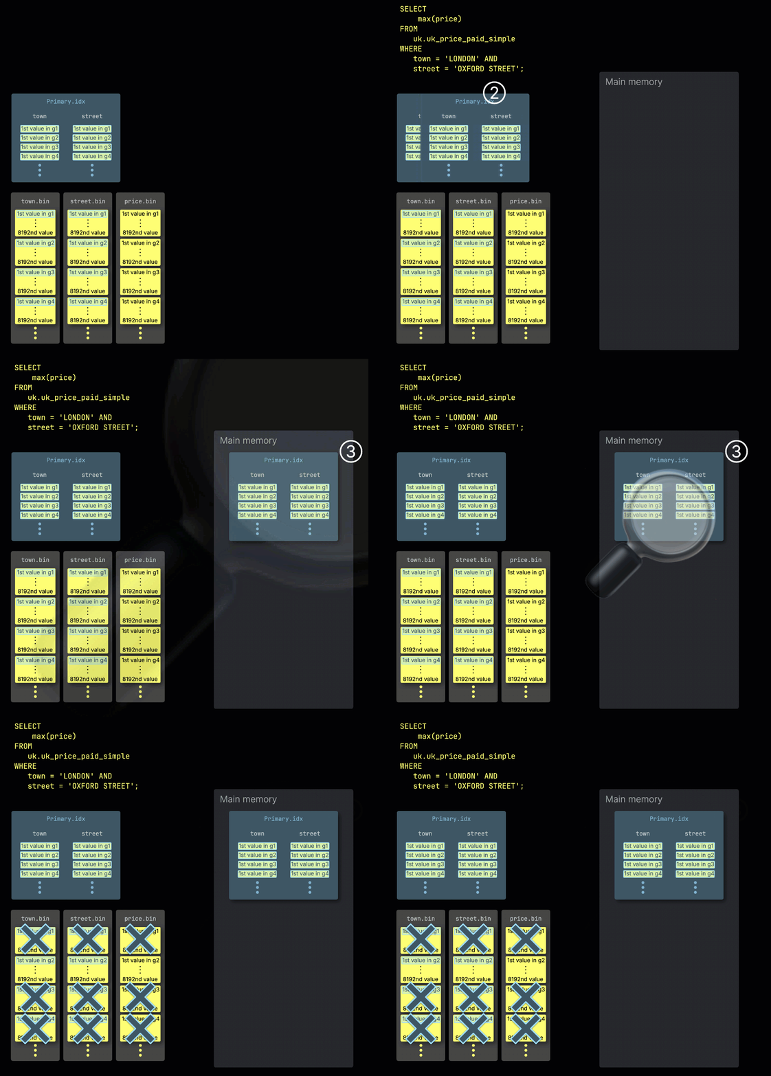
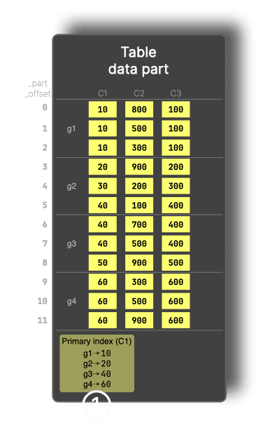
Index-based pruning: skip granules that cannot match the predicate
ClickHouse Blog
Parallel replicas coordinator distributing work across nodes
ClickHouse Blog
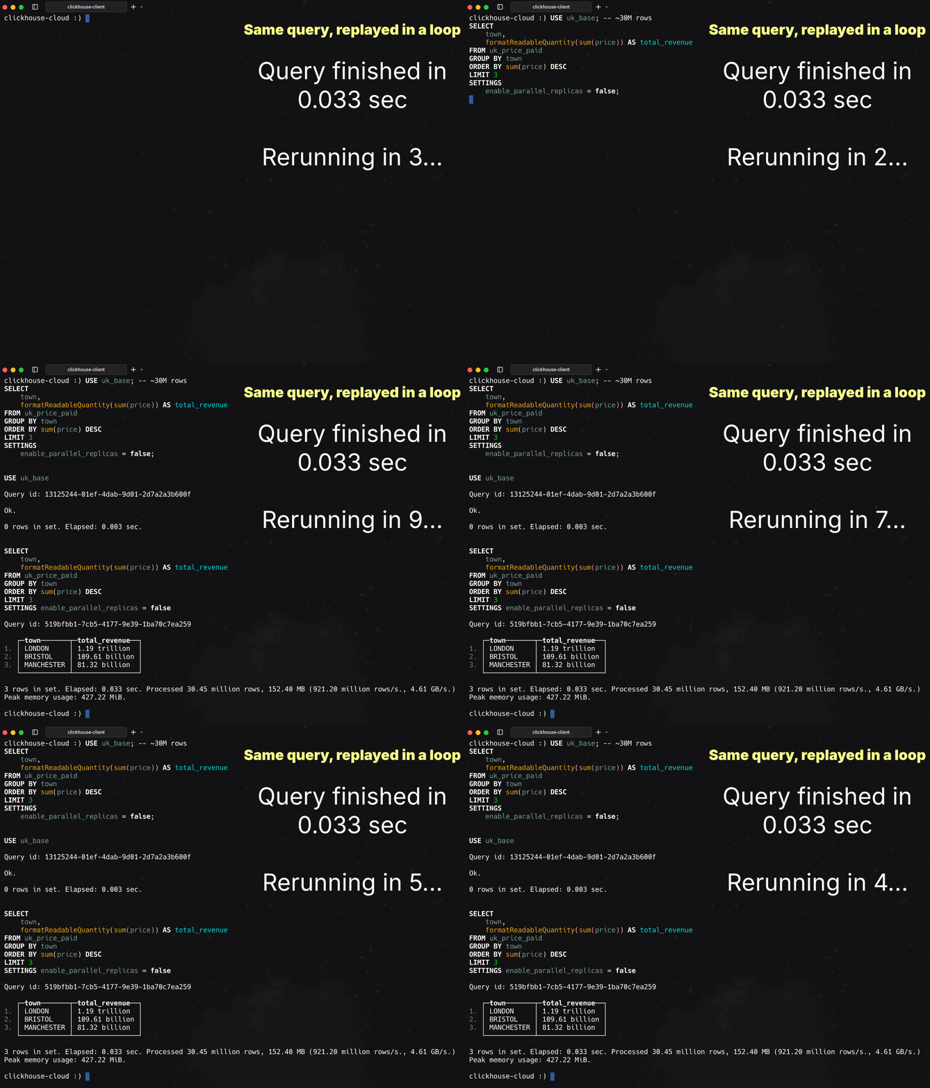
Animated GIF: parallel-replicas GROUP BY finishing in 33 ms
📚 Full module reference
Module 6 — Query Optimisation & Performance
Audience: anyone making CH queries fast — or wondering why theirs
aren't. Prerequisites: Modules 1–2. Time: ~75 min reading + 30
min hands-on with measurable timings on 60M rows.
By the end you will be able to:
Read a CH query plan (EXPLAIN, EXPLAIN SYNTAX, EXPLAIN PIPELINE,
EXPLAIN PROJECTION, EXPLAIN indexes = 1).
Diagnose performance from system.query_log and system.parts.
Choose ORDER BY, PRIMARY KEY, projections, and skip-indexes for the
workload.
Use PREWHERE and SAMPLE correctly.
Pick between ANY, ALL, ASOF, and dictionary JOINs.
Build a Materialized View that pre-aggregates at write time.
1. The query lifecycle
💬 Discuss with AI — click to view prompt
Paste into ChatGPT, Claude, Gemini, or any LLM chat.
I'm studying ClickHouse and working through the module "ClickHouse Query Optimization". I want to deeply understand the section: "The query lifecycle".

Here is a brief excerpt from the material I'm reading:

"""
What you actually tune at each step: | Stage          | Knobs you control                                                                  | | Reader         | `ORDER BY`, `PARTITION BY`, projections, skip-indexes, `PREWHERE`, `SAMPLE`         | | Optimizer      | settings (`optimize_read_in_order`, `optimize_use_projections`, JIT, `compile_aggregate_expressions`) | | Pipeline       | `max_threads`, `max_memory_usage`, parallel replicas                                | | Result         | `max_block_size`, format choice                                                     |
"""

Please explain this concept in depth. Cover:

1. **Core mechanics** — how does it actually work under the hood? What data structures, algorithms, or engine internals are involved? Where is the implementation in the ClickHouse source tree (file/folder names) if you know?

2. **When to use vs avoid** — what concrete workloads does this help, and when would it hurt or be wrong? Give specific scale/latency trade-offs.

3. **Comparable features in other systems** — how does this compare with similar features in PostgreSQL, MySQL, BigQuery, Snowflake, Redshift, or DuckDB? Build my intuition by analogy.

4. **Common pitfalls and gotchas** — what trips engineers up in production? Subtle bugs, performance traps, surprising semantics?

5. **Worked example** — show me a small but realistic SQL or config example that demonstrates the concept end-to-end. Include the expected output where useful.

6. **Where to read more** — a short list of authoritative pointers (CH docs, blog posts, talks, source-code files).

Assume I have solid SQL fundamentals but I'm new to ClickHouse internals. Be technical but pragmatic; avoid marketing language.
What you actually tune at each step:
Stage
Knobs you control
Reader
ORDER BY, PARTITION BY, projections, skip-indexes, PREWHERE, SAMPLE
2. The first thing to check: did the engine read what you think it did?
💬 Discuss with AI — click to view prompt
Paste into ChatGPT, Claude, Gemini, or any LLM chat.
I'm studying ClickHouse and working through the module "ClickHouse Query Optimization". I want to deeply understand the section: "The first thing to check: did the engine read what you think it did?".

Here is a brief excerpt from the material I'm reading:

"""
**`read_rows` is the truth.** If your `WHERE` filter looks selective but `read_rows ≈ total table size`, the index didn't help. `SYSTEM FLUSH LOGS;` first if the table is empty — `query_log` is flushed periodically (~7.5 s default), not synchronously.
"""

Please explain this concept in depth. Cover:

1. **Core mechanics** — how does it actually work under the hood? What data structures, algorithms, or engine internals are involved? Where is the implementation in the ClickHouse source tree (file/folder names) if you know?

2. **When to use vs avoid** — what concrete workloads does this help, and when would it hurt or be wrong? Give specific scale/latency trade-offs.

3. **Comparable features in other systems** — how does this compare with similar features in PostgreSQL, MySQL, BigQuery, Snowflake, Redshift, or DuckDB? Build my intuition by analogy.

4. **Common pitfalls and gotchas** — what trips engineers up in production? Subtle bugs, performance traps, surprising semantics?

5. **Worked example** — show me a small but realistic SQL or config example that demonstrates the concept end-to-end. Include the expected output where useful.

6. **Where to read more** — a short list of authoritative pointers (CH docs, blog posts, talks, source-code files).

Assume I have solid SQL fundamentals but I'm new to ClickHouse internals. Be technical but pragmatic; avoid marketing language.
SELECT
    query_duration_ms,
    read_rows,
    formatReadableSize(read_bytes) AS read_bytes,
    formatReadableSize(memory_usage) AS mem,
    result_rows
FROM system.query_log
WHERE event_time > now() - INTERVAL 5 MINUTE
  AND type = 'QueryFinish'
ORDER BY event_time DESC LIMIT 10;
read_rows is the truth. If your WHERE filter looks selective but
read_rows ≈ total table size, the index didn't help.
SYSTEM FLUSH LOGS; first if the table is empty — query_log is
flushed periodically (~7.5 s default), not synchronously.
3. ORDER BY shape — where almost every win comes from
💬 Discuss with AI — click to view prompt
Paste into ChatGPT, Claude, Gemini, or any LLM chat.
I'm studying ClickHouse and working through the module "ClickHouse Query Optimization". I want to deeply understand the section: "ORDER BY shape — where almost every win comes from".

Here is a brief excerpt from the material I'm reading:

"""
The same 20M rows, three table layouts (this is what the demo tests): | Layout                                    | Filter `WHERE event_time BETWEEN 'a' AND 'b'`    | Filter `WHERE country = 'US'` | | `ORDER BY (event_type, country)`          | full scan (no time prefix in PK)                 | partial via secondary scan    | | `ORDER BY (event_time, user_id)`          | granule pruning → reads ~1/30th                  | full scan, scans by date      | | `ORDER BY (event_time, user_id)` + projection on `(country, day)` | granule pruning            | reads from projection (tiny)  | ### How to c...
"""

Please explain this concept in depth. Cover:

1. **Core mechanics** — how does it actually work under the hood? What data structures, algorithms, or engine internals are involved? Where is the implementation in the ClickHouse source tree (file/folder names) if you know?

2. **When to use vs avoid** — what concrete workloads does this help, and when would it hurt or be wrong? Give specific scale/latency trade-offs.

3. **Comparable features in other systems** — how does this compare with similar features in PostgreSQL, MySQL, BigQuery, Snowflake, Redshift, or DuckDB? Build my intuition by analogy.

4. **Common pitfalls and gotchas** — what trips engineers up in production? Subtle bugs, performance traps, surprising semantics?

5. **Worked example** — show me a small but realistic SQL or config example that demonstrates the concept end-to-end. Include the expected output where useful.

6. **Where to read more** — a short list of authoritative pointers (CH docs, blog posts, talks, source-code files).

Assume I have solid SQL fundamentals but I'm new to ClickHouse internals. Be technical but pragmatic; avoid marketing language.
The same 20M rows, three table layouts (this is what the demo tests):
Layout
Filter WHERE event_time BETWEEN 'a' AND 'b'
Filter WHERE country = 'US'
ORDER BY (event_type, country)
full scan (no time prefix in PK)
partial via secondary scan
ORDER BY (event_time, user_id)
granule pruning → reads ~1/30th
full scan, scans by date
ORDER BY (event_time, user_id) + projection on (country, day)
granule pruning
reads from projection (tiny)
How to choose
What's the most common WHERE filter? That column should be the
first in ORDER BY. Time-series workloads almost always lead with
event_time or its truncation (toStartOfHour(event_time)).
What's the most common GROUP BY? Putting that column second
enables optimize_aggregation_in_order.
High-cardinality columns later in the key.user_id after
event_time is fine; event_time after user_id would scatter
adjacent rows in time across the file.
4. Projections — second copies optimised for a different shape
💬 Discuss with AI — click to view prompt
Paste into ChatGPT, Claude, Gemini, or any LLM chat.
I'm studying ClickHouse and working through the module "ClickHouse Query Optimization". I want to deeply understand the section: "Projections — second copies optimised for a different shape".

Here is a brief excerpt from the material I'm reading:

"""
Projections are *managed-by-the-engine* materialised aggregations / sort orders that live alongside the main part. What happens: - Every part now also stores a projection part (a tiny aggregated sub-table). - A query of the right shape reads from the projection, not the base table. - Triggered automatically when `optimize_use_projections = 1` (default) *and* the query matches. | Win                                                          | Cost                              | | Aggregation queries 10–100× faster                           | Projection storage ≈ size of the aggregate result × nu...
"""

Please explain this concept in depth. Cover:

1. **Core mechanics** — how does it actually work under the hood? What data structures, algorithms, or engine internals are involved? Where is the implementation in the ClickHouse source tree (file/folder names) if you know?

2. **When to use vs avoid** — what concrete workloads does this help, and when would it hurt or be wrong? Give specific scale/latency trade-offs.

3. **Comparable features in other systems** — how does this compare with similar features in PostgreSQL, MySQL, BigQuery, Snowflake, Redshift, or DuckDB? Build my intuition by analogy.

4. **Common pitfalls and gotchas** — what trips engineers up in production? Subtle bugs, performance traps, surprising semantics?

5. **Worked example** — show me a small but realistic SQL or config example that demonstrates the concept end-to-end. Include the expected output where useful.

6. **Where to read more** — a short list of authoritative pointers (CH docs, blog posts, talks, source-code files).

Assume I have solid SQL fundamentals but I'm new to ClickHouse internals. Be technical but pragmatic; avoid marketing language.
Projections are managed-by-the-engine materialised aggregations / sort
orders that live alongside the main part.
CREATE TABLE events_proj (
    event_time DateTime,
    user_id    UInt64,
    country    LowCardinality(String),
    amount     Float64,

    PROJECTION pv_country_day (
        SELECT country, toDate(event_time) AS day,
               count(), sum(amount), avg(amount)
        GROUP BY country, day
    )
)
ENGINE = MergeTree
ORDER BY (event_time, user_id);
What happens:
- Every part now also stores a projection part (a tiny aggregated
sub-table).
- A query of the right shape reads from the projection, not the base
table.
- Triggered automatically when optimize_use_projections = 1 (default)
and the query matches.
EXPLAIN PROJECTION = 1
SELECT country, toDate(event_time) AS day, count()
FROM events_proj
WHERE event_time BETWEEN '2026-02-01' AND '2026-02-28'
GROUP BY country, day;
-- Plan should mention "Projection: pv_country_day"
Win
Cost
Aggregation queries 10–100× faster
Projection storage ≈ size of the aggregate result × number of parts
No application changes
Mutations rewrite the projection too
Multiple projections per table
Slower writes (each projection is computed)
5. Skip indexes — granule pruning for the second column
💬 Discuss with AI — click to view prompt
Paste into ChatGPT, Claude, Gemini, or any LLM chat.
I'm studying ClickHouse and working through the module "ClickHouse Query Optimization". I want to deeply understand the section: "Skip indexes — granule pruning for the second column".

Here is a brief excerpt from the material I'm reading:

"""
Skip indexes prune **granules**, not rows. A skip index on column X is useful when X *isn't* in the PK prefix but you filter on it. | Type                    | Stores                              | Best for                                  | | `minmax`                | min, max per N granules             | Range filters on numeric/date columns     | | `set(K)`                | up to K distinct values per N granules | `IN` / `=` on low-cardinality columns  | | `bloom_filter`          | bloom filter per N granules         | High-cardinality `=` filters (like `user_id`) | | `tokenbf_v1(L, K, S)`...
"""

Please explain this concept in depth. Cover:

1. **Core mechanics** — how does it actually work under the hood? What data structures, algorithms, or engine internals are involved? Where is the implementation in the ClickHouse source tree (file/folder names) if you know?

2. **When to use vs avoid** — what concrete workloads does this help, and when would it hurt or be wrong? Give specific scale/latency trade-offs.

3. **Comparable features in other systems** — how does this compare with similar features in PostgreSQL, MySQL, BigQuery, Snowflake, Redshift, or DuckDB? Build my intuition by analogy.

4. **Common pitfalls and gotchas** — what trips engineers up in production? Subtle bugs, performance traps, surprising semantics?

5. **Worked example** — show me a small but realistic SQL or config example that demonstrates the concept end-to-end. Include the expected output where useful.

6. **Where to read more** — a short list of authoritative pointers (CH docs, blog posts, talks, source-code files).

Assume I have solid SQL fundamentals but I'm new to ClickHouse internals. Be technical but pragmatic; avoid marketing language.
Skip indexes prune granules, not rows. A skip index on column X is
useful when X isn't in the PK prefix but you filter on it.
Type
Stores
Best for
minmax
min, max per N granules
Range filters on numeric/date columns
set(K)
up to K distinct values per N granules
IN / = on low-cardinality columns
bloom_filter
bloom filter per N granules
High-cardinality = filters (like user_id)
tokenbf_v1(L, K, S)
per-token bloom filter
Substring search via hasToken()
ngrambf_v1(N, L, K, S)
per-ngram bloom filter
LIKE searches with %abc%
CREATE TABLE events_idx (
    event_time DateTime,
    user_id    UInt64,
    country    LowCardinality(String),
    amount     Float64,
    url        String,

    INDEX idx_amount  amount  TYPE minmax        GRANULARITY 4,
    INDEX idx_country country TYPE set(100)      GRANULARITY 4,
    INDEX idx_user    user_id TYPE bloom_filter() GRANULARITY 4,
    INDEX idx_url_tok url     TYPE tokenbf_v1(8192, 3, 0) GRANULARITY 4
)
ENGINE = MergeTree ORDER BY (event_time, user_id);
GRANULARITY = 4 means "one index entry per 4 marks" — i.e. one entry per
~32k rows. Higher granularity = smaller index, less precise; lower = larger.
A skip index never produces wrong results. It just might fail to
prune (false positives in bloom filters → still read the granule). If
your queries don't filter on the indexed column, the index is dead weight
on writes — drop it.
6. PREWHERE — read less
💬 Discuss with AI — click to view prompt
Paste into ChatGPT, Claude, Gemini, or any LLM chat.
I'm studying ClickHouse and working through the module "ClickHouse Query Optimization". I want to deeply understand the section: "PREWHERE — read less".

Here is a brief excerpt from the material I'm reading:

"""
CH automatically rewrites cheap predicates into `PREWHERE`, which reads the predicate columns first, prunes granules, and only then reads the remaining columns. You'd write `PREWHERE` explicitly when: - The optimiser picks the wrong predicate to push down (rare on modern CH). - You want to *guarantee* the order: cheap filter first, expensive later. `EXPLAIN SYNTAX` shows what the optimiser actually did:
"""

Please explain this concept in depth. Cover:

1. **Core mechanics** — how does it actually work under the hood? What data structures, algorithms, or engine internals are involved? Where is the implementation in the ClickHouse source tree (file/folder names) if you know?

2. **When to use vs avoid** — what concrete workloads does this help, and when would it hurt or be wrong? Give specific scale/latency trade-offs.

3. **Comparable features in other systems** — how does this compare with similar features in PostgreSQL, MySQL, BigQuery, Snowflake, Redshift, or DuckDB? Build my intuition by analogy.

4. **Common pitfalls and gotchas** — what trips engineers up in production? Subtle bugs, performance traps, surprising semantics?

5. **Worked example** — show me a small but realistic SQL or config example that demonstrates the concept end-to-end. Include the expected output where useful.

6. **Where to read more** — a short list of authoritative pointers (CH docs, blog posts, talks, source-code files).

Assume I have solid SQL fundamentals but I'm new to ClickHouse internals. Be technical but pragmatic; avoid marketing language.
CH automatically rewrites cheap predicates into PREWHERE, which reads
the predicate columns first, prunes granules, and only then reads the
remaining columns.
-- These are equivalent on CH 21+:
SELECT count() FROM events WHERE country = 'US' AND amount > 100;
SELECT count() FROM events PREWHERE country = 'US' WHERE amount > 100;
You'd write PREWHERE explicitly when:
The optimiser picks the wrong predicate to push down (rare on modern CH).
You want to guarantee the order: cheap filter first, expensive later.
EXPLAIN SYNTAX shows what the optimiser actually did:
EXPLAIN SYNTAX
SELECT count() FROM events WHERE country = 'US' AND amount > 100;
7. SAMPLE — orders-of-magnitude faster, with caveats
💬 Discuss with AI — click to view prompt
Paste into ChatGPT, Claude, Gemini, or any LLM chat.
I'm studying ClickHouse and working through the module "ClickHouse Query Optimization". I want to deeply understand the section: "SAMPLE — orders-of-magnitude faster, with caveats".

Here is a brief excerpt from the material I'm reading:

"""
`SAMPLE` reads a *consistent fraction* of rows. Requires `SAMPLE BY` in the table definition. | Use SAMPLE for                     | Don't use SAMPLE for                                       | | Real-time dashboards over fresh data | Exact-count metrics                                       | | `quantile`, `avg`, `count` approximations | Reports auditors will scrutinise                      | | Iterative exploration              | Joins (sampling on both sides is hard to reason about)     |
"""

Please explain this concept in depth. Cover:

1. **Core mechanics** — how does it actually work under the hood? What data structures, algorithms, or engine internals are involved? Where is the implementation in the ClickHouse source tree (file/folder names) if you know?

2. **When to use vs avoid** — what concrete workloads does this help, and when would it hurt or be wrong? Give specific scale/latency trade-offs.

3. **Comparable features in other systems** — how does this compare with similar features in PostgreSQL, MySQL, BigQuery, Snowflake, Redshift, or DuckDB? Build my intuition by analogy.

4. **Common pitfalls and gotchas** — what trips engineers up in production? Subtle bugs, performance traps, surprising semantics?

5. **Worked example** — show me a small but realistic SQL or config example that demonstrates the concept end-to-end. Include the expected output where useful.

6. **Where to read more** — a short list of authoritative pointers (CH docs, blog posts, talks, source-code files).

Assume I have solid SQL fundamentals but I'm new to ClickHouse internals. Be technical but pragmatic; avoid marketing language.
SAMPLE reads a consistent fraction of rows. Requires SAMPLE BY in
the table definition.
CREATE TABLE events_sampled (
    ...
)
ENGINE = MergeTree
ORDER BY (event_time, intHash32(user_id), user_id)
SAMPLE BY intHash32(user_id);

SELECT count() * 10, avg(amount) FROM events_sampled SAMPLE 0.1;
-- ≈ 10× faster, ~10× variance
Use SAMPLE for
Don't use SAMPLE for
Real-time dashboards over fresh data
Exact-count metrics
quantile, avg, count approximations
Reports auditors will scrutinise
Iterative exploration
Joins (sampling on both sides is hard to reason about)
8. JOIN strategies
💬 Discuss with AI — click to view prompt
Paste into ChatGPT, Claude, Gemini, or any LLM chat.
I'm studying ClickHouse and working through the module "ClickHouse Query Optimization". I want to deeply understand the section: "JOIN strategies".

Here is a brief excerpt from the material I'm reading:

"""
CH joins are *generally* slower than its scans. Pick wisely. | Join type         | Right-side cardinality | Left-side cardinality | Behaviour                                          | | `INNER JOIN`      | small                  | any                   | Hash-build right, stream left.                     | | `LEFT/RIGHT JOIN` | small                  | any                   | Same; null-fill non-matches.                       | | `ANY LEFT JOIN`   | any                    | any                   | First match per left row. Faster than ALL.         | | `ALL LEFT JOIN`   | any...
"""

Please explain this concept in depth. Cover:

1. **Core mechanics** — how does it actually work under the hood? What data structures, algorithms, or engine internals are involved? Where is the implementation in the ClickHouse source tree (file/folder names) if you know?

2. **When to use vs avoid** — what concrete workloads does this help, and when would it hurt or be wrong? Give specific scale/latency trade-offs.

3. **Comparable features in other systems** — how does this compare with similar features in PostgreSQL, MySQL, BigQuery, Snowflake, Redshift, or DuckDB? Build my intuition by analogy.

4. **Common pitfalls and gotchas** — what trips engineers up in production? Subtle bugs, performance traps, surprising semantics?

5. **Worked example** — show me a small but realistic SQL or config example that demonstrates the concept end-to-end. Include the expected output where useful.

6. **Where to read more** — a short list of authoritative pointers (CH docs, blog posts, talks, source-code files).

Assume I have solid SQL fundamentals but I'm new to ClickHouse internals. Be technical but pragmatic; avoid marketing language.
CH joins are generally slower than its scans. Pick wisely.
Join type
Right-side cardinality
Left-side cardinality
Behaviour
INNER JOIN
small
any
Hash-build right, stream left.
LEFT/RIGHT JOIN
small
any
Same; null-fill non-matches.
ANY LEFT JOIN
any
any
First match per left row. Faster than ALL.
ALL LEFT JOIN
any
any
Cartesian on duplicates (default behaviour).
ASOF LEFT JOIN
any
any
Match nearest-but-not-after on a continuous column.
Dictionary lookup
tiny (< 100M rows)
huge
Best-of-class for small dim tables.
Dictionary as a JOIN replacement
CREATE DICTIONARY users_dict (
    user_id UInt64,
    cohort  String,
    signup_date Date
)
PRIMARY KEY user_id
SOURCE(CLICKHOUSE(host 'localhost' port 9000 db 'm6' table 'users_dim'))
LIFETIME(MIN 60 MAX 300)
LAYOUT(HASHED());

SYSTEM RELOAD DICTIONARY m6.users_dict;

-- Now lookups are RAM-resident hashmap reads:
SELECT count(),
       avgIf(amount, dictGetString('m6.users_dict', 'cohort', user_id) = 'alpha')
FROM events_good;
Layout
RAM
Lookup speed
Use for
HASHED
high
fastest
< 50M small rows
SPARSE_HASHED
medium
fast
< 200M rows
RANGE_HASHED
medium
fast
versioned dim with date ranges
IP_TRIE
low
fast
IPv4/IPv6 ranges
CACHE
configurable
medium
huge dims, slower miss path
DIRECT
none
slow
always queries the source
9. Materialized Views for query optimisation
💬 Discuss with AI — click to view prompt
Paste into ChatGPT, Claude, Gemini, or any LLM chat.
I'm studying ClickHouse and working through the module "ClickHouse Query Optimization". I want to deeply understand the section: "Materialized Views for query optimisation".

Here is a brief excerpt from the material I'm reading:

"""
A MV pre-computes aggregates **at INSERT time**. Read latency is then a function of the MV's row count, not the source's. Reads from `country_daily` are millions of times smaller than from `events_good`. Module 2 covers MV semantics in depth.
"""

Please explain this concept in depth. Cover:

1. **Core mechanics** — how does it actually work under the hood? What data structures, algorithms, or engine internals are involved? Where is the implementation in the ClickHouse source tree (file/folder names) if you know?

2. **When to use vs avoid** — what concrete workloads does this help, and when would it hurt or be wrong? Give specific scale/latency trade-offs.

3. **Comparable features in other systems** — how does this compare with similar features in PostgreSQL, MySQL, BigQuery, Snowflake, Redshift, or DuckDB? Build my intuition by analogy.

4. **Common pitfalls and gotchas** — what trips engineers up in production? Subtle bugs, performance traps, surprising semantics?

5. **Worked example** — show me a small but realistic SQL or config example that demonstrates the concept end-to-end. Include the expected output where useful.

6. **Where to read more** — a short list of authoritative pointers (CH docs, blog posts, talks, source-code files).

Assume I have solid SQL fundamentals but I'm new to ClickHouse internals. Be technical but pragmatic; avoid marketing language.
A MV pre-computes aggregates at INSERT time. Read latency is then a
function of the MV's row count, not the source's.
CREATE TABLE country_daily (
    day Date, country LowCardinality(String),
    events UInt64, revenue Float64
) ENGINE = SummingMergeTree ORDER BY (day, country);

CREATE MATERIALIZED VIEW country_daily_mv TO country_daily AS
SELECT toDate(event_time) AS day, country,
       count() AS events, sum(amount) AS revenue
FROM events_good
GROUP BY day, country;

-- Backfill once
INSERT INTO country_daily
SELECT toDate(event_time), country, count(), sum(amount)
FROM events_good GROUP BY toDate(event_time), country;
Reads from country_daily are millions of times smaller than from
events_good. Module 2 covers MV semantics in depth.
10. The EXPLAIN family
💬 Discuss with AI — click to view prompt
Paste into ChatGPT, Claude, Gemini, or any LLM chat.
I'm studying ClickHouse and working through the module "ClickHouse Query Optimization". I want to deeply understand the section: "The EXPLAIN family".

Here is a brief excerpt from the material I'm reading:

"""
(no excerpt — section heading was "The EXPLAIN family")
"""

Please explain this concept in depth. Cover:

1. **Core mechanics** — how does it actually work under the hood? What data structures, algorithms, or engine internals are involved? Where is the implementation in the ClickHouse source tree (file/folder names) if you know?

2. **When to use vs avoid** — what concrete workloads does this help, and when would it hurt or be wrong? Give specific scale/latency trade-offs.

3. **Comparable features in other systems** — how does this compare with similar features in PostgreSQL, MySQL, BigQuery, Snowflake, Redshift, or DuckDB? Build my intuition by analogy.

4. **Common pitfalls and gotchas** — what trips engineers up in production? Subtle bugs, performance traps, surprising semantics?

5. **Worked example** — show me a small but realistic SQL or config example that demonstrates the concept end-to-end. Include the expected output where useful.

6. **Where to read more** — a short list of authoritative pointers (CH docs, blog posts, talks, source-code files).

Assume I have solid SQL fundamentals but I'm new to ClickHouse internals. Be technical but pragmatic; avoid marketing language.
Form
Shows
EXPLAIN
Plan tree (the default).
EXPLAIN AST
Raw parser AST.
EXPLAIN SYNTAX
Query as the optimiser rewrote it (PREWHERE pushdown, alias inlining).
EXPLAIN PIPELINE
The actual pipeline (operators, threads, branches).
EXPLAIN PIPELINE graph = 1
DOT format; pipe to graphviz for a picture.
EXPLAIN PLAN actions = 1
Per-operator action list — every projection/filter/aggregate.
EXPLAIN indexes = 1
Which indexes (PK, partition, skip) the planner used.
EXPLAIN PROJECTION = 1
Whether a projection got picked.
EXPLAIN ESTIMATE
Estimated rows/parts/granules to read.
EXPLAIN indexes = 1
SELECT count() FROM events_proj WHERE user_id = 12345;
-- Looks for: "Skip index: idx_user (bloom_filter)"
11. The hands-on demo
💬 Discuss with AI — click to view prompt
Paste into ChatGPT, Claude, Gemini, or any LLM chat.
I'm studying ClickHouse and working through the module "ClickHouse Query Optimization". I want to deeply understand the section: "The hands-on demo".

Here is a brief excerpt from the material I'm reading:

"""
### What you get ### Three layouts of the same 20M rows ### Execution flow — what runs, in order | #  | Step          | What happens                                                                                                                                                                                                            | | 0  | self-bootstrap | If `m6-clickhouse` isn't healthy, `up.sh` brings it up. The container is given a 6 GB memory limit because the dataset is large.                                                                                       | | 1  | `setup.sql`...
"""

Please explain this concept in depth. Cover:

1. **Core mechanics** — how does it actually work under the hood? What data structures, algorithms, or engine internals are involved? Where is the implementation in the ClickHouse source tree (file/folder names) if you know?

2. **When to use vs avoid** — what concrete workloads does this help, and when would it hurt or be wrong? Give specific scale/latency trade-offs.

3. **Comparable features in other systems** — how does this compare with similar features in PostgreSQL, MySQL, BigQuery, Snowflake, Redshift, or DuckDB? Build my intuition by analogy.

4. **Common pitfalls and gotchas** — what trips engineers up in production? Subtle bugs, performance traps, surprising semantics?

5. **Worked example** — show me a small but realistic SQL or config example that demonstrates the concept end-to-end. Include the expected output where useful.

6. **Where to read more** — a short list of authoritative pointers (CH docs, blog posts, talks, source-code files).

Assume I have solid SQL fundamentals but I'm new to ClickHouse internals. Be technical but pragmatic; avoid marketing language.
If m6-clickhouse isn't healthy, up.sh brings it up. The container is given a 6 GB memory limit because the dataset is large.
1
setup.sql
Creates database m6 and three identically-shaped tables: events_bad (wrong PK), events_good (right PK), events_proj (right PK + bloom-filter on user_id + projection on (country, day)).
2
data.sql
Inserts 20M rows into events_good, then INSERT INTO bad/proj SELECT * FROM events_good so all three tables hold identical data. OPTIMIZE FINAL on each so timings aren't muddied by background merges. ~30–60s.
3
queries.sql
Five comparisons: time-range count on each layout (Q1), country aggregation on each (Q2 — projection should crush), point lookup by user_id (Q3 — skip index helps), EXPLAIN indexes=1 and EXPLAIN PROJECTION=1 (Q4), then SYSTEM FLUSH LOGS + system.query_log summary (Q5).
4
extras.sql
More tools: PREWHERE (auto + explicit, with EXPLAIN SYNTAX), SAMPLE BY intHash32(user_id) table copy and SAMPLE 0.1 query, three more skip-index types (minmax, set, tokenbf_v1), JOIN strategies (ANY vs ALL vs Dictionary lookup) against a 500k-row users_dim, and a Materialized View (country_daily_mv → country_daily SummingMergeTree) with a backfill.
What you should observe
The exact numbers depend on hardware; the ratios are stable. On an
M-series MacBook the demo typically prints:
Query
BAD ordering
GOOD ordering
PROJ + skip idx
Q1 — time range
scans most parts
reads few granules
reads few granules
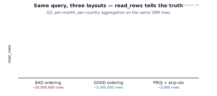
Q2 — country aggregation per month
~1.8 s, ~20M read
~0.25 s, ~5M read
~0.02 s, ~3k read
Q3 — point lookup by user_id
scans all rows
scans all rows
bloom filter prunes most marks
12. Settings worth knowing for query work
💬 Discuss with AI — click to view prompt
Paste into ChatGPT, Claude, Gemini, or any LLM chat.
I'm studying ClickHouse and working through the module "ClickHouse Query Optimization". I want to deeply understand the section: "Settings worth knowing for query work".

Here is a brief excerpt from the material I'm reading:

"""
| Setting                                | Default | Effect                                                              | | `max_threads`                          | cores  | Per-query parallelism.                                              | | `max_memory_usage`                     | 10 GB  | Per-query memory cap. Aggregations OOM here.                        | | `max_bytes_before_external_group_by`   | 0      | If > 0, spill GROUP BY to disk above this size.                     | | `optimize_read_in_order`               | 1      | Skip sort if PK already orders the data....
"""

Please explain this concept in depth. Cover:

1. **Core mechanics** — how does it actually work under the hood? What data structures, algorithms, or engine internals are involved? Where is the implementation in the ClickHouse source tree (file/folder names) if you know?

2. **When to use vs avoid** — what concrete workloads does this help, and when would it hurt or be wrong? Give specific scale/latency trade-offs.

3. **Comparable features in other systems** — how does this compare with similar features in PostgreSQL, MySQL, BigQuery, Snowflake, Redshift, or DuckDB? Build my intuition by analogy.

4. **Common pitfalls and gotchas** — what trips engineers up in production? Subtle bugs, performance traps, surprising semantics?

5. **Worked example** — show me a small but realistic SQL or config example that demonstrates the concept end-to-end. Include the expected output where useful.

6. **Where to read more** — a short list of authoritative pointers (CH docs, blog posts, talks, source-code files).

Assume I have solid SQL fundamentals but I'm new to ClickHouse internals. Be technical but pragmatic; avoid marketing language.
Setting
Default
Effect
max_threads
cores
Per-query parallelism.
max_memory_usage
10 GB
Per-query memory cap. Aggregations OOM here.
max_bytes_before_external_group_by
0
If > 0, spill GROUP BY to disk above this size.
optimize_read_in_order
1
Skip sort if PK already orders the data.
optimize_aggregation_in_order
0
Stream aggregation when PK matches GROUP BY prefix.
optimize_use_projections
1
Try to match a projection.
compile_aggregate_expressions
1
JIT-compile aggregate functions.
parallel_replicas_for_non_replicated_merge_tree
0
Allow parallel replicas mode even on non-replicated tables.
max_block_size
65536
Rows per pipeline block. Bigger = more memory, fewer overhead bumps.
13. Common pitfalls
💬 Discuss with AI — click to view prompt
Paste into ChatGPT, Claude, Gemini, or any LLM chat.
I'm studying ClickHouse and working through the module "ClickHouse Query Optimization". I want to deeply understand the section: "Common pitfalls".

Here is a brief excerpt from the material I'm reading:

"""
| Symptom                                                                | Cause                                                                                | Fix                                                                                              | | `WHERE date_col = '2026-05-01'` reads everything                       | `date_col` not in PK prefix; or filter on `toDate(date_col)` while PK is `DateTime`. | Match the type/expression exactly. Use a function-index or partition key.                        | | Projection isn't picked                                                | Que...
"""

Please explain this concept in depth. Cover:

1. **Core mechanics** — how does it actually work under the hood? What data structures, algorithms, or engine internals are involved? Where is the implementation in the ClickHouse source tree (file/folder names) if you know?

2. **When to use vs avoid** — what concrete workloads does this help, and when would it hurt or be wrong? Give specific scale/latency trade-offs.

3. **Comparable features in other systems** — how does this compare with similar features in PostgreSQL, MySQL, BigQuery, Snowflake, Redshift, or DuckDB? Build my intuition by analogy.

4. **Common pitfalls and gotchas** — what trips engineers up in production? Subtle bugs, performance traps, surprising semantics?

5. **Worked example** — show me a small but realistic SQL or config example that demonstrates the concept end-to-end. Include the expected output where useful.

6. **Where to read more** — a short list of authoritative pointers (CH docs, blog posts, talks, source-code files).

Assume I have solid SQL fundamentals but I'm new to ClickHouse internals. Be technical but pragmatic; avoid marketing language.
Symptom
Cause
Fix
WHERE date_col = '2026-05-01' reads everything
date_col not in PK prefix; or filter on toDate(date_col) while PK is DateTime.
Match the type/expression exactly. Use a function-index or partition key.
Projection isn't picked
Query shape doesn't match projection.
EXPLAIN PROJECTION = 1 to see why. Reshape the query or add another projection.
Bloom-filter index doesn't help
Granularity too coarse; or column has high collision rate.
Lower GRANULARITY; verify with EXPLAIN indexes = 1.
Memory limit (for query) exceeded
Aggregation cardinality > max_memory_usage.
Set max_bytes_before_external_group_by to spill to disk.
Same query is fast once, slow on second run
Filesystem page cache cold the first time, hot the second.
Benchmark with SYSTEM DROP MARK CACHE and SYSTEM DROP UNCOMPRESSED CACHE between runs.
JOIN is slow
Right-hand side too big.
Use a Dictionary; pre-aggregate; or use IN (SELECT ...) with SETTINGS distributed_product_mode='global'.
SAMPLE returns wildly different counts on re-runs
Forgot SAMPLE BY in the table definition; SAMPLE became a no-op or random.
SHOW CREATE TABLE and add SAMPLE BY ....
14. Talking points for the live session
💬 Discuss with AI — click to view prompt
Paste into ChatGPT, Claude, Gemini, or any LLM chat.
I'm studying ClickHouse and working through the module "ClickHouse Query Optimization". I want to deeply understand the section: "Talking points for the live session".

Here is a brief excerpt from the material I'm reading:

"""
1. **`read_rows` is your X-ray machine.** Show before/after on the same query. 2. **`ORDER BY` is the highest-leverage knob.** Run Q1 on the `BAD` and `GOOD` tables side-by-side and watch the ratio. 3. **Projections are not free.** They add write-time cost but query-time wins are 10–100×. 4. **Skip indexes prune granules, not rows.** Show `idx_user` on a point lookup; `EXPLAIN indexes = 1` shows the prune. 5. **PREWHERE is auto.** `EXPLAIN SYNTAX` reveals it. Don't write it unless the optimiser picks wrong. 6. **Dictionary > JOIN** for small dim tables. Demo with the 500k-row `users_dim`. 7. *...
"""

Please explain this concept in depth. Cover:

1. **Core mechanics** — how does it actually work under the hood? What data structures, algorithms, or engine internals are involved? Where is the implementation in the ClickHouse source tree (file/folder names) if you know?

2. **When to use vs avoid** — what concrete workloads does this help, and when would it hurt or be wrong? Give specific scale/latency trade-offs.

3. **Comparable features in other systems** — how does this compare with similar features in PostgreSQL, MySQL, BigQuery, Snowflake, Redshift, or DuckDB? Build my intuition by analogy.

4. **Common pitfalls and gotchas** — what trips engineers up in production? Subtle bugs, performance traps, surprising semantics?

5. **Worked example** — show me a small but realistic SQL or config example that demonstrates the concept end-to-end. Include the expected output where useful.

6. **Where to read more** — a short list of authoritative pointers (CH docs, blog posts, talks, source-code files).

Assume I have solid SQL fundamentals but I'm new to ClickHouse internals. Be technical but pragmatic; avoid marketing language.
read_rows is your X-ray machine. Show before/after on the same
query.
ORDER BY is the highest-leverage knob. Run Q1 on the BAD and
GOOD tables side-by-side and watch the ratio.
Projections are not free. They add write-time cost but query-time
wins are 10–100×.
Skip indexes prune granules, not rows. Show idx_user on a point
lookup; EXPLAIN indexes = 1 shows the prune.
PREWHERE is auto.EXPLAIN SYNTAX reveals it. Don't write it
unless the optimiser picks wrong.
Dictionary > JOIN for small dim tables. Demo with the 500k-row
users_dim.
Materialized Views finish the job. Once a query is materialised,
it's microseconds regardless of source size.
15. Going deeper
💬 Discuss with AI — click to view prompt
Paste into ChatGPT, Claude, Gemini, or any LLM chat.
I'm studying ClickHouse and working through the module "ClickHouse Query Optimization". I want to deeply understand the section: "Going deeper".

Here is a brief excerpt from the material I'm reading:

"""
- **Module 2** — Materialized Views in detail. - **Module 3** — distributed query plans. - **CH docs**: <https://clickhouse.com/docs/en/optimize/query-optimization> - **Profile-guided optimisation:** load `system.query_log` into a separate table, then aggregate by query pattern to find your top offenders.
"""

Please explain this concept in depth. Cover:

1. **Core mechanics** — how does it actually work under the hood? What data structures, algorithms, or engine internals are involved? Where is the implementation in the ClickHouse source tree (file/folder names) if you know?

2. **When to use vs avoid** — what concrete workloads does this help, and when would it hurt or be wrong? Give specific scale/latency trade-offs.

3. **Comparable features in other systems** — how does this compare with similar features in PostgreSQL, MySQL, BigQuery, Snowflake, Redshift, or DuckDB? Build my intuition by analogy.

4. **Common pitfalls and gotchas** — what trips engineers up in production? Subtle bugs, performance traps, surprising semantics?

5. **Worked example** — show me a small but realistic SQL or config example that demonstrates the concept end-to-end. Include the expected output where useful.

6. **Where to read more** — a short list of authoritative pointers (CH docs, blog posts, talks, source-code files).

Assume I have solid SQL fundamentals but I'm new to ClickHouse internals. Be technical but pragmatic; avoid marketing language.